
CLIENT STORY
The client is an apparel manufacturer based in Europe. Its seasonal collections go out through several sales channels, and every style comes in a long list of colors and sizes. With 2 seasonal collections a year and 4 sales channels, the catalog ran to more than 1,500 SKUs. Lead times in production were long, too, so a wrong call on a committed batch was hard to fix. Leadership wanted to stop basing production quantities on a planner’s best guess from last season’s numbers and have them follow actual demand instead.
| Service: | Data Analytics |
|---|---|
| Industry: | Manufacturing |
| Year: | 2025 |
| Region: | EU |
| Cooperation type: | Ongoing Partnership |
Read summarized version with


We'd overproduce one style and run out of another in the same week, and by the time anyone noticed, the batch that could have fixed it was already three weeks into production. — Head of Production Planning
Every line changeover we could plan ahead of time was setup time and trial runs we didn't have to pay for. — Plant Manager
The Challenge: A Forecast That Couldn't Keep Up
The catalog was big: more than 1,500 SKUs across seasonal collections, sizes, colors, and four sales channels. Still, size was only part of what made forecasting hard. Demand for one style could look very different in another color, size, or channel. Promotions, price changes, and new product launches kept moving it as well, so historical averages became less and less reliable.
For production planning, the team still worked mostly in Excel, from last season’s sales plus planner judgment. Every update was done by hand, and demand across product variants moved faster than that. One style could be gone within weeks while another was still in the warehouse at the next markdown cycle.
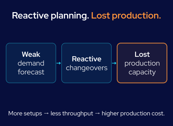
Behind the stock problem sat a second cost. Changing a line over to a different style, fabric, or color between production runs took setup time, and while a line was being set up, it wasn’t producing. Reliable demand forecasts would have let production teams group compatible runs ahead of time. Without them, schedules often changed on short notice.
Long lead times made it worse. A forecast that was off early in the season didn’t show up as a problem until weeks later: an empty rack, or an unsold pallet. By then there was rarely time left to correct course.
A Hybrid AI Forecasting System for Production Planning
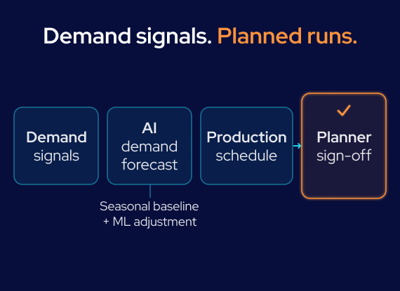
GroupBWT chose a hybrid forecasting approach over separate forecasts based only on historical sales. Seasonal patterns that recur came first; machine-learning adjustments for pricing, promotions, product attributes, and recent demand signals went on top. For planners, that meant seeing demand change early enough to adjust production schedules before a stock imbalance got expensive.
A Seasonal Baseline for Every Style Family. Layer one learned the recurring side of demand: seasonality, trend, holiday effects, and the patterns that repeat across related style families. GroupBWT pulled historical sales, orders, inventory, SKU attributes, pricing, promotions, and calendar data into one forecasting pipeline that ran the same way every time. New styles were trickier, since they had no sales history at all. For those, the system borrowed from comparable product families, shared attributes, price bands, and the track record of similar products. Once a style launched, its early sell-through became another input for updating the forecast.
An AI/ML Layer for Demand Deviations. The second layer was where the ML came in. GroupBWT trained gradient-boosted models to predict when actual demand would likely drift from the seasonal baseline. The feature set covered price changes, promotions, regional weather patterns, sales channel, product attributes, recent sell-through, and SKU-specific demand behavior. Nothing replaced the seasonal model. The ML layer merged those signals with the baseline into a forecast for each individual product variant, and shifted it wherever demand looked set to break from what the baseline alone predicted.
From AI Forecast to Production Plan. The SKU-level forecasts then got rolled up to style-family level, the level production planning works at, and turned into batch requirements and production runs the plant could actually schedule. GroupBWT sequenced those runs so compatible styles, fabrics, and colors ran back to back. Fewer unnecessary line changeovers, less idle setup time. No run got recommended until the scheduling layer had checked forecasted demand against current inventory levels, available capacity, production lead times, batch constraints, and existing orders. Even then, a planner reviewed the recommendation and could override it (more on that below).
Operationally, the forecast always covered the next 12 weeks. A weekly refresh with new sales, inventory, and sell-through data meant mid-season demand shifts showed up fast, with no need to lean on a forecast made once before launch. Until a production run inside those 12 weeks was committed, its batch size, replenishment volume, and line allocation stayed open, and planners could change any of them. That’s how slow-moving variants got cut back and faster-selling ones got more supply. Committed runs already in progress were a different matter; they stayed on the manufacturer’s existing production lead times. Most weekly adjustments changed batch quantities and line allocation inside runs that were already grouped but not yet committed; the style and color sequence wasn’t reshuffled every week. For anything beyond that window, the longer-term seasonal plans kept guiding material and capacity commitments.
Backtested Against Historical Demand Before Production Use
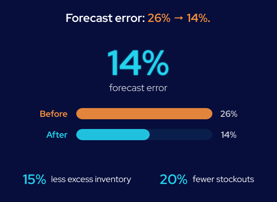
Tested Before Production Decisions Relied on It. First came a backtest. GroupBWT ran the model on historical periods it had never seen in training and lined its results up against the manufacturer’s previous planning baseline, using the same evaluation window and forecast horizon. Scoring was done per style family, because that’s the level production-volume and batch decisions were made at. SKU-level forecasts were still there for replenishment and stockout monitoring. Scored that way, WAPE dropped from 26% to 14%. WAPE stands for weighted absolute percentage error: it tells you how far the forecast landed from actual demand. Forecast bias was on the watch list too, to make sure the model wasn’t running consistently high or low on demand.
One Forecasting Pipeline for Inventory and Production Planning. Replenishment decisions at SKU level, plus production and capacity planning at aggregated levels, all came out of one forecasting pipeline. That put planners and plant managers on the same demand numbers.
Human-in-the-Loop, Not Fully Automatic. Nothing became a production order without a planner having the chance to override it first. The model proposed the default; if it clearly missed something, a person made the final call.
Tech stack: Python, XGBoost, time-series seasonal decomposition, feature engineering pipeline, rolling forecast pipeline, WAPE and forecast-bias monitoring, production scheduling logic, planning dashboard
A forecast that only lives in a dashboard doesn't save you a line changeover. The value showed up once expected demand started shaping the actual production sequence, not just telling planners what to expect.

Forecast Error Cut From 26% to 14%, With Less Excess Inventory and Fewer Stockouts
Historical backtesting showed that the new forecasting approach reduced WAPE from 26% to 14% at the style-family level, compared with the manufacturer’s previous planning method, before a single production order relied on it. The inventory and stockout figures below come from a separate measurement: the system’s first season running in production, against the previous comparable season.
- By aligning production quantities with that more accurate forecast instead of a planner’s estimate, GroupBWT helped the manufacturer carry 15% less excess inventory on slow-moving styles, sizes, and colors compared with the previous comparable season.
- By flagging demand shifts early enough in the season to still act on them, GroupBWT helped the manufacturer cut stockouts on fast-moving SKUs by 20% compared with the previous comparable season.
- By grouping compatible styles and colors into longer, better-sequenced production runs, GroupBWT helped the manufacturer reduce its average number of weekly line changeovers by roughly 30% over that same first season.
Still Planning Production Around Last Season's Demand?
We help manufacturers take demand forecasts all the way into production plans, which means fewer stockouts, less excess inventory, and fewer reactive production changes. Book a forecasting assessment to see where better demand signals could improve your production plan.




You have an idea?
We handle all the rest.
How can we help you?